MultiHeadAttention (MHA)
Principle
Query (Q),Key (K), andValue (V)are all projected intonum_headsindependent heads- The dimension per head
head_dimishidden_size // num_heads - Each Query head calculates attention
Attentionwith corresponding Key/Value heads completely independently
Advantages
- ✅ High expressiveness, each head can learn different semantic subspaces (e.g., syntax, coreference, position, etc.)
Disadvantages
- ❌ High memory and computational overhead: Storage and computation for K/V linearly increase with
H. - ❌ During long-sequence inference, KV Cache consumes massive VRAM (e.g., 32k context)
import torch
from torch import nn
import math

class MultiHeadAttention(nn.Module):
    def __init__(self, hidden_size, num_heads):
        super(MultiHeadAttention, self).__init__()
        assert hidden_size % num_heads == 0, "hidden_size must be divisible by num_heads."
        self.num_heads = num_heads
        self.head_dim = hidden_size // num_heads
        self.q_linear = nn.Linear(hidden_size, hidden_size) # IN: hidden_size, OUT: hidden_size
        self.k_linear = nn.Linear(hidden_size, hidden_size) # IN: hidden_size, OUT: hidden_size
        self.v_linear = nn.Linear(hidden_size, hidden_size) # IN: hidden_size, OUT: hidden_size
        self.o_linear = nn.Linear(hidden_size, hidden_size) # IN: hidden_size, OUT: hidden_size

    def split_heads(self, x):
        """
        Split into MultiHead
        (batch_size, seq_len, hidden_size) → (batch_size, num_heads, seq_len, head_dim)
        """
        batch_size, seq_len, _ = x.size()
        x = x.view(batch_size, seq_len, self.num_heads, self.head_dim) # Split the last dimension (hidden_size) logically into (num_heads, head_dim) | (batch_size, seq_len, hidden_size) → (batch_size, seq_len, num_heads, head_dim)
        return x.transpose(1, 2)  # Swap the second dimension (seq_len) and the third dimension (num_heads) | (batch_size, seq_len, num_heads, head_dim) → (batch_size, num_heads, seq_len, head_dim)

    def combine_heads(self, x):
        """
        Combine MultiHead
        (batch, num_heads, seq_len, head_dim) → (batch, seq_len, hidden)
        """
        batch_size, _, seq_len, _ = x.size()
        x = x.transpose(1, 2).contiguous()  # (batch_size, num_heads, seq_len, head_dim) → (batch_size, seq_len, num_heads, head_dim)
        return x.view(batch_size, seq_len, -1)  # → (batch_size, seq_len, hidden_size)

    def forward(self, hidden_state, attention_mask=None):
        batch_size = hidden_state.size(0)

        # hidden_state: (batch_size, seq_len, hidden_size)

        # STEP 1. Linear Projection
        Q = self.q_linear(hidden_state) # (batch_size, seq_len, hidden_size)
        K = self.k_linear(hidden_state)
        V = self.v_linear(hidden_state)

        # STEP 2. Split into MultiHead
        Q = self.split_heads(Q)  # (batch_size, num_heads, seq_len, head_dim)
        K = self.split_heads(K)
        V = self.split_heads(V)

        # STEP 3. Calculate Attention Score: QK^T / sqrt(d_k)
        # Q: (batch_size, num_heads, seq_len, head_dim)
        # K^T: (batch_size, num_heads, head_dim, seq_len)
        # matmul → (batch_size, num_heads, seq_len, seq_len)
        scale = math.sqrt(self.head_dim)
        scores = torch.matmul(Q, K.transpose(-2, -1)) / scale

        # STEP 4. Apply mask
        if attention_mask is not None:
            if attention_mask.dim() == 2:
                attention_mask = attention_mask.unsqueeze(1).unsqueeze(2) # (batch_size, seq_len) → (batch_size, 1, 1, seq_len)
            scores = scores.masked_fill(attention_mask == 1, float('-inf'))

        # STEP 5. Softmax + Weighted Sum
        attn_probs = torch.softmax(scores, dim=-1)  # (batch_size, num_heads, seq_len, seq_len)
        output = torch.matmul(attn_probs, V)        # (batch_size, num_heads, seq_len, seq_len) * (batch_size, num_heads, seq_len, head_dim) → (batch_size, num_heads, seq_len, head_dim)

        # STEP 6. Combine MultiHead
        output = self.combine_heads(output)  # (batch_size, seq_len, hidden_size)
        output = self.o_linear(output)       # MultiHead(Q, K, V) = Concat(head₁, ..., headₕ) · Wᴼ where headᵢ = Attention(QWᵢ^Q, KWᵢ^K, VWᵢ^V)

        return output
Multi-Query Attention (MQA)
Principle
Query (Q)retainsnum_headsheadsKey (K)andValue (V)use only1head- All
Query (Q)heads share the same set of K/V - Utilize PyTorch's broadcasting mechanism to automatically align dimensions
Advantages
- ✅ Significantly reduced KV Cache memory: From
2 × H × L × d→2 × 1 × L × d(savingHtimes) - ✅ Faster inference speed, especially suitable for long text generation
Disadvantages
- ❌ Reduced expressiveness: All Query heads share the same contextual representation, potentially丢失 fine-grained information.
- ❌ Training may converge slightly slower or require hyperparameter tuning
import torch
from torch import nn
import math

class MultiQueryAttention(nn.Module):
    def __init__(self, hidden_size, num_heads):
        super(MultiQueryAttention, self).__init__()
        assert hidden_size % num_heads == 0, "hidden_size must be divisible by num_heads"
        self.num_heads = num_heads
        self.head_dim = hidden_size // num_heads
        self.q_linear = nn.Linear(hidden_size, hidden_size) # IN: hidden_size, OUT: hidden_size
        self.k_linear = nn.Linear(hidden_size, self.head_dim)  # IN: hidden_size, OUT: hidden_size // num_heads
        self.v_linear = nn.Linear(hidden_size, self.head_dim)  # IN: hidden_size, OUT: hidden_size // num_heads
        self.o_linear = nn.Linear(hidden_size, hidden_size) # IN: hidden_size, OUT: hidden_size

    def _split_heads(self, x, n_heads):
        batch_size, seq_len, _ = x.size()
        x = x.view(batch_size, seq_len, n_heads, self.head_dim)
        return x.transpose(1, 2)  # (B, n_heads, L, d)

    def forward(self, hidden_state, attention_mask=None):
        batch_size = hidden_state.size(0)

        # hidden_state: (batch_size, seq_len, hidden_size)

        # STEP 1. Linear Projection
        Q = self.q_linear(hidden_state) # (batch_size, seq_len, hidden_size)
        K = self.k_linear(hidden_state) # (batch_size, seq_len, head_dim)
        V = self.v_linear(hidden_state) # (batch_size, seq_len, head_dim)
        # STEP 2. Split into MultiHead
        Q = self._split_heads(Q, self.num_heads) # (batch_size, num_heads, seq_len, head_dim)
        K = self._split_heads(K, 1) # (batch_size, 1, seq_len, head_dim)
        V = self._split_heads(V, 1) # (batch_size, 1, seq_len, head_dim)

        # STEP 3. Calculate Attention Score: QK^T / sqrt(d_k)
        # Q: (batch_size, num_heads, seq_len, head_dim)
        # K: (batch_size, 1, seq_len, head_dim)
        # K^T: (batch_size, 1, head_dim, seq_len)
        # matmul → (batch_size, num_heads, seq_len, seq_len) ✅ Broadcasting successful (1 → H)
        scale = math.sqrt(self.head_dim)
        scores = torch.matmul(Q, K.transpose(-2, -1)) / scale

        # STEP 4. Apply mask
        if attention_mask is not None:
            if attention_mask.dim() == 2:
                attention_mask = attention_mask.unsqueeze(1).unsqueeze(2)
            scores = scores.masked_fill(attention_mask == 1, float('-inf'))

        # STEP 5. Softmax + Weighted Sum
        attn_probs = torch.softmax(scores, dim=-1)
        output = torch.matmul(attn_probs, V) # (batch_size, num_heads, seq_len, seq_len) * (batch_size, num_heads, seq_len, head_dim) → (batch_size, num_heads, seq_len, head_dim)

        # STEP 6. Combine MultiHead
        # output: (batch_size, num_heads, seq_len, head_dim)
        # transpose → (batch_size, seq_len, num_heads, head_dim)
        # view → (batch_size, seq_len, num_heads*head_dim)
        output = output.transpose(1, 2).contiguous()
        output = output.view(batch_size, -1, self.num_heads * self.head_dim)
        output = self.o_linear(output)
        return output
Grouped-Query Attention (GQA)
Principle
Query (Q)hasnum_headsheadsKey (K)andValue (V)havegroup_numheads (1 < group_num < num_heads), andnum_heads % group_num == 0- Every
num_heads // group_numQuery heads share a set of K/V
Advantages
- ✅ Balances MHA and MQA: Strikes a compromise between expressiveness and efficiency
- ✅ Significantly reduces KV Cache memory: Reduces by
H / Gtimes (e.g., halved if G=2) - ✅ Empirical performance close to MHA, far superior to MQA (proposed by Google, used in PaLM-2)
Disadvantages
- ❌ Implementation is slightly complex (requires handling grouped broadcasting)
- ❌ Need to choose an appropriate
group_num(typically 2~8)
import torch
from torch import nn
import math

class GroupQueryAttention(nn.Module):
    def __init__(self, hidden_size, num_heads, group_num):
        super(GroupQueryAttention, self).__init__()
        assert num_heads % group_num == 0, "num_heads must be divisible by group_num"
        self.num_heads = num_heads
        self.group_num = group_num
        self.head_dim = hidden_size // num_heads
        self.q_linear = nn.Linear(hidden_size, num_heads * self.head_dim) # IN: hidden_size, OUT: hidden_size
        self.k_linear = nn.Linear(hidden_size, group_num * self.head_dim) # IN: hidden_size, OUT: group_num * head_dim
        self.v_linear = nn.Linear(hidden_size, group_num * self.head_dim) # IN: hidden_size, OUT: group_num * head_dim
        self.o_linear = nn.Linear(num_heads * self.head_dim, hidden_size) # IN: hidden_size, OUT: hidden_size

    def _split_heads(self, x, n_heads):
        batch_size, seq_len, _ = x.size()
        x = x.view(batch_size, seq_len, n_heads, self.head_dim)
        return x.transpose(1, 2)

    def forward(self, hidden_state, attention_mask=None):
        batch_size = hidden_state.size(0)

        # STEP 1. Linear Projection
        Q = self.q_linear(hidden_state) # (batch_size, seq_len, hidden_size)
        K = self.k_linear(hidden_state) # (batch_size, seq_len, group_num * head_dim)
        V = self.v_linear(hidden_state) # (batch_size, seq_len, group_num * head_dim)

        # STEP 2. Split into MultiHead
        Q = self._split_heads(Q, self.num_heads) # (batch_size, num_heads, seq_len, head_dim)
        K = self._split_heads(K, self.group_num) # (batch_size, group_num, seq_len, head_dim)
        V = self._split_heads(V, self.group_num) # (batch_size, group_num, seq_len, head_dim)

        # 3. ★ GQA Core: Broadcast Key/Value to each group of Query heads ★
        # Each group has `num_heads // group_num` query heads sharing the same K/V group
        # Example: H_q=8, H_g=2 → each group has 4 query heads sharing 1 K/V group
        # Method: Repeat K/V along the head dimension, NOT reshape!
        repeat_times = self.num_heads // self.group_num
        K = K.unsqueeze(2).expand(-1, -1, repeat_times, -1, -1).reshape(
            batch_size, self.num_heads, -1, self.head_dim
        )
        V = V.unsqueeze(2).expand(-1, -1, repeat_times, -1, -1).reshape(
            batch_size, self.num_heads, -1, self.head_dim
        )

        scale = math.sqrt(self.head_dim)
        scores = torch.matmul(Q, K.transpose(-2, -1)) / scale

        # STEP 4. Apply mask
        if attention_mask is not None:
            if attention_mask.dim() == 2:
                attention_mask = attention_mask.unsqueeze(1).unsqueeze(2)
            scores = scores.masked_fill(attention_mask == 1, float('-inf'))

        # STEP 5. Softmax + Weighted Sum
        attn_probs = torch.softmax(scores, dim=-1)
        output = torch.matmul(attn_probs, V)

        # STEP 6. Combine MultiHead
        output = output.transpose(1, 2).contiguous()
        output = output.view(batch_size, -1, self.num_heads * self.head_dim)
        output = self.o_linear(output)
        return output
MHA & GQA & MQA Comparison
| Feature | MHA | GQA | MQA |
|---|---|---|---|
| KV Heads Count | H | G (1 < G < H) | 1 |
| Query Heads Count | H | H | H |
| KV Cache Memory | 2 × H × L × d | 2 × G × L × d | 2 × L × d |
| Expressiveness | ⭐⭐⭐⭐⭐ | ⭐⭐⭐⭐ | ⭐⭐⭐ |
| Inference Speed | Slow | Medium | Fast |
| Training Stability | High | High | Medium (may require tuning) |
| Typical Applications | BERT, ViT | PaLM-2, Mixtral | StarCoder, T5, LLaMA (some) |
Multi-Head Latent Attention (MLA)
Cache: Shadow Circles
Cache: Green Bandwidth Font

- : Model hidden dimension (hidden size)
- : Number of attention heads (number of heads)
- : Dimension per head
- : KV compression latent vector dimension (e.g., 512)
- : Q compression latent vector dimension (e.g., 1536)
- : RoPE component head dimension (e.g., 64)
1. KV Compression and Reconstruction
Input token representation
KV Compression (Shared)
KV Reconstruction
2. RoPE Components
RoPE Key (Shared) (MQA style)
RoPE Components for Query (per-head)
First compress Q:
Then generate RoPE Q:
Can be reshaped into:
3. Q/K/V Construction
Query
First reconstruct the content part of Q:
Concatenate RoPE:
Key
Value
4. Attention Calculation
Score
Attention
Output
5. Multi-head Combination
Matrix Absorption
When calculating :
The dot product is:
Where:
- is a fixed parameter and can be precomputed
→ During inference, there is no need to reconstruct ; simply cache .
Similarly, can be absorbed into , avoiding the need to explicitly cache .
| Cached Item | Dimension | Description |
|---|---|---|
| Low-rank latent vector (e.g., 512) | ||
| RoPE Key (MQA, e.g., 56) |
Native Sparse Attention (NSA)
Summary of NSA in one sentence
NSA = Compress to see global first → Select to see local second → Add sliding window to preserve proximity → Fuse three outputs via gating. Learning sparsity from the start is far more reliable than post-hoc pruning.
Detailed Explanation of the Three Attention Branches
Overview
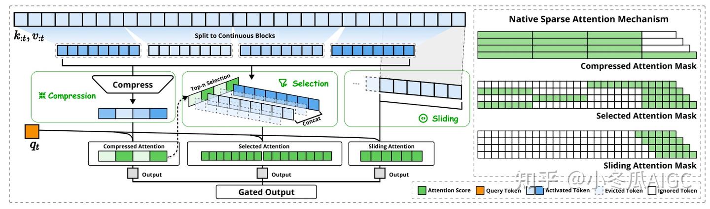
Input sequence x₁, x₂, ..., x_T
         │
         ↓
   Linear projection → Q, K, V
         │
    ┌────┼────────────┐
    ↓    ↓            ↓
  Compress  Select      Sliding
  Attention  Attention    Attention
    │    ↑            │
    │    │            │
    │  Compression     │
    │  score → top-k   │
    │  block selection │
    ↓    ↓            ↓
  o_cmp  o_slc      o_win  Dimensions are the same!
    │    │            │
    └────┼────────────┘
         │
   Gating Fusion: g_cmp·o_cmp + g_slc·o_slc + g_win·o_win
         │
         ↓
      Final output o*
1. 🔵 Compression Attention
Objective: Quickly scan the entire document to find "roughly which sections are important."
Method: Compress a segment of KVs into a single KV.
Original KV sequence (32 tokens):
[k₁,k₂,k₃,k₄,k₅,k₆,k₇,k₈ | k₉,...,k₁₆ | k₁₇,...,k₂₄ | k₂₅,...,k₃₂]
          Block 1             Block 2          Block 3         Block 4

Compressed (4 tokens):
[k̃₁, k̃₂, k̃₃, k̃₄]
  ↑     ↑     ↑     ↑
  Block 1    Block 2   Block 3   Block 4 "Representatives"
How to compress? Use an MLP (small neural network):
Compress 8 Ks into 1 K̃:
K̃₁ = MLP(k₁, k₂, k₃, k₄, k₅, k₆, k₇, k₈)
This is like summarizing 8 sentences into 1 sentence—losing details but retaining the gist.
Then Q computes attention only with the 4 compressed Ks:
Q₃₂ · K̃₁ = 0.5   ← Block 1 not important
Q₃₂ · K̃₂ = 2.8   ← Block 2 is important! ★
Q₃₂ · K̃₃ = 0.3   ← Block 3 not important
Q₃₂ · K̃₄ = 3.1   ← Block 4 is important! ★
Output of Compression Attention: Fuses global information from 4 blocks (coarse, but comprehensive).
2. 🟢 Selection Attention
Objective: Finely read "important blocks" discovered by compression attention.
Method: Based on compression attention scores, select top-k blocks and retrieve original full KVs to compute.
Compression finds: Block 2 and Block 4 are important

Then retrieve original KVs for Block 2 and Block 4:
K₂ = [k₉, k₁₀, ..., k₁₆]  ← 8 Ks
K₄ = [k₂₅, k₂₆, ..., k₃₂] ← 8 Ks

Q₃₂ computes attention with these 16 Ks → fine-grained local information
Output of Selection Attention: Finely fuses information only from important blocks (precise, but local).
3. 🟡 Sliding Window Attention
Objective: Ensure nearby tokens are always attended to.
Method: Take the nearest w KV tokens and compute attention directly.
Q₃₂ computes attention only with the nearest 8 KVs:
[k₂₅, k₂₆, k₂₇, k₂₈, k₂₉, k₃₀, k₃₁, k₃₂]
Why is this needed? Because compression and selection might miss crucial neighboring information.
For example, the referent of a pronoun like "he" is usually among the preceding few tokens. This relationship cannot be captured by global scanning alone.
4. 🔴 Gating Fusion
After computing three at
Final output = g_cmp × o_cmp + g_slc × o_slc + g_win × o_win
This is like:
- Abstract/Summary accounts for 30% (Compressed)
- Core Chapters account for 50% (Selected)
- Contextual Continuity accounts for 20% (Sliding Window)
And these proportions are learned by the model itself, varying from token to token.
Compression Ratio and Complexity Analysis
Numerical Sensation
Context length T = 65536 (64K):
| Attention Type | KV Count | Source |
|---|---|---|
| Compression Attention | 128 | T/l = 65536/512 |
| Selection Attention | 4096 | 8 blocks × 512 |
| Sliding Window Attention | 4096 | Window size w |
| NSA Total | 8320 | |
| Standard Attention | 65536 | All KVs |
Complexity Trend as Sequence Length Increases
| Scheme | Computational Complexity | When T Doubles |
|---|---|---|
| Standard Attention | O(T²) | Computation ×4 |
| NSA | ≈ O(T·B_c + T·k·l + T·w) | Computation ≈ ×2 |
- (number of compressed blocks) = T/l → Linear growth
- (number of selected blocks) = Fixed constant
- (sliding window size) = Fixed constant
As , NSA computation tends to grow linearly, while standard attention grows quadratically. The larger T is, the more apparent NSA's advantage becomes.
Does Sparsification Cause Information Loss?
Mitigation Mechanism 1: Multi-layer Overlap Coverage
Layer 1 NSA: Selects [Block 1, Block 3]
Layer 2 NSA: Selects [Block 2, Block 3]
Layer 3 NSA: Selects [Block 1, Block 4]

→ After 3 layers, all 4 blocks are covered
Mitigation Mechanism 2: Information Propagation Layer by Layer
Layer 1: Q₃₂ fuses information from Block 1 and Block 3 → Output o₃₂
                │
                ↓ Residual Connection + FFN
Layer 2: o₃₂ becomes Layer 2's K₃₂, V₃₂

So Layer 2's K₃₂ already "knows" the content of Block 1 and Block 3!
Even if Layer 2 only selects Block 2, it can indirectly obtain information from Block 1 via K₃₂.
Relationship with MLA / GQA
| Scheme | Application Point | Problem Solved | Mechanism |
|---|---|---|---|
| MLA | Wk/Wv projection layers | KV-Cache storage too large | Low-rank compression of KV projection |
| GQA | Attention head structure | Too many KV heads | Multi-head Q shares single-head KV |
| NSA | Attention calculation layer | Attention computation too large | Sparsification of KV sequence |
┌─────────────────────────────────────────┐
│  Input token x                            │
│         │                                │
│  ┌─── Projection Layer ───┐                        │
│  │  Wq, Wk, Wv   │ ← MLA here          │
│  │  (Low-rank compressed KV)  │    Reduce KV storage volume       │
│  └───────────────┘                        │
│         ↓ Q, K, V                         │
│  ┌─── Head Structure ───┐                        │
│  │  MHA/GQA/MQA  │ ← GQA here          │
│  │  (Multi-head Q shares KV) │    Reduce KV head count           │
│  └───────────────┘                        │
│         ↓ Split Q, K, V                        │
│  ┌─── Attention Calculation ─┐                      │
│  │  Standard/NSA  │ ← NSA here        │
│  │  (Select KV then compute)  │    Reduce KVs participating in computation │
│  └─────────────────┘                     │
└─────────────────────────────────────────┘

All three can be stacked: MLA + GQA + NSA = Low storage + Low heads + Low computation
DeepSeek Sparse Attention (DSA)
1. Why DSA Exists
- The pain points of NSA are Block-wise and Native:
- Block-wise granularity is too coarse: NSA adopts a block-based strategy for selecting KVs. However, attention distribution in long texts is often scattered and fine-grained (Element-wise). Forcing block division leads to accuracy degradation, or to maintain accuracy, one must retain excessively large blocks, reducing sparsification efficiency.
- Native pretraining cannot be compatible with existing strong baselines: NSA requires models to undergo "native pretraining" from scratch. However, DeepSeek at this time already possesses an extremely powerful
V3.1-Terminusdense (Dense) large model base. If we abandon the mature base and train from scratch just for sparsification, the computational cost and risk are extremely high.
2. DSA Core Architecture Design
The essence of DSA is: Before entering the expensive standard attention calculation, use extremely low cost to help each Query Token filter out the most valuable Top-K (constant, e.g., 2048) KV Tokens from the entire sequence.
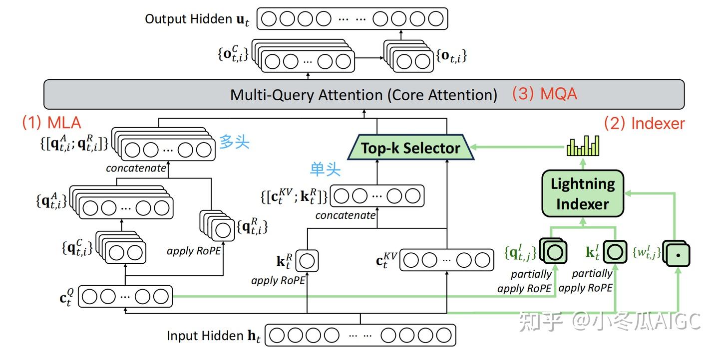
① Lightning Indexer (Lightweight Indexing Network)
Calculation Formula:
Low-cost filtering: The Indexer possesses independent projection matrices. It amplifies the main model's Latent into multi-head (total of 64 heads), while projecting input into a single shared head for all heads (MAQ downsampling idea).
Non-linear Gating: Utilizes to learn importance weights for each head, and applies
ReLUactivation (instead of standard Softmax). The entire Indexer's computation is only about 1/9 of the main model's MLA. Finally, throughTop-Koperation, it directly extracts 2048 fine-grained historical token indices.
② MQA (Multi-Query Attention) Equivalent Transformation
Why MQA? Even if 2048 tokens are selected, if during KV Cache retrieval from HBM (VRAM) to SRAM (high-speed cache), the data is still restored to a conventional multi-head (e.g., 128 heads) dimension, it still creates a massive memory access bottleneck.
Equivalent Transformation: Leveraging the low-rank compression properties inherent to MLA (Multi-head Latent Attention), the main model uses MHA during Prefill (phase) to guarantee computational parallelism, but during Decoding (phase), it can elegantly transform it into an MQA mechanism using the associativity of matrix multiplication.
Result: KV Cache data volume drops drastically when loaded into SRAM (128 heads become 1 head, data volume becomes 1/128). MQA reduces memory traffic data volume, while DSA reduces computational load; the two form a powerful dual strategy.
③ Token-wise Mask (Fine-grained Mask Control)
In engineering implementation, DSA does not dynamically crop matrices because non-aligned matrix multiplications are extremely difficult to optimize on GPUs.
- DSA's method: After the Indexer selects Top-K indices, it generates an
index_maskof matrix size. - Assign (negative infinity) to unselected positions, and to selected positions.
- Overlay this Mask directly onto Attention Scores for
Softmax, thereby mathematically implicitly removing non-Top-K tokens. Coupled with underlying Triton/CUDA Kernel optimizations, skipping calculations at positions.
3. DSA Smoothly Inherits from Dense Base
1. Dense Warm-up Phase
- Strategy: Freeze the main model, train only the Lightning Indexer for 1000 steps. The main model still follows traditional full Dense Attention.
- Objective: Let the newly initialized Indexer learn and align with the main model's attention distribution.
- Training signal source: KL Divergence Loss, using the main model's full Attention scores as the Target, guiding the Indexer's output to approximate it.
2. Sparse Training Phase
- Strategy: Release all parameters (main model + Indexer), formally introduce Top-K fine-grained filtering, and calculate only sparse attention.
- Objective: Allow the main model and Indexer to jointly adapt to the sparse new norm of "only seeing 2048 tokens."
- Training signal source: Joint Loss; the Indexer continues to align via KL Divergence on locally selected tokens; the main model focuses on optimizing Cross-Entropy Loss for language modeling.
Ref "Associativity of Multiplication" Transformation
The formula for standard MHA Attention Score is:
- is multi-head (dimension
[1, 128, 576]) - is also multi-head (dimension
[Len, 128, 576]) - To calculate it, you must pull out the large matrix from VRAM during Decode.
DeepSeek's MLA introduced the concept of Low-rank Compression. When DeepSeek generates , it does not generate it directly, but obtains it by multiplying a low-rank compressed vector (a single shared vector of extremely low dimension) with an upscaling matrix :
So, the original calculation formula can be rewritten as:
Now, Associativity of Multiplication takes the stage!
- Approach A (Calculate as is): First let restore into multi-head . This is the MHA mode.
Cost: If done during Decode, every historical token's multi-head must be stored or restored in VRAM, causing a 128-fold explosion in data volume and instantly bombarding memory bandwidth.
- Approach B (Utilize Associativity): Since the formula is , and during Decode the current is only 1 (and known), why not let multiply with first?
- Before entering attention calculation, pre-multiply the current with the upscaling matrix and fuse them into a temporary intermediate variable .
- Next, we only need to read that single compressed vector from VRAM!
- Calculation becomes: .
Compressed Sparse Attention (CSA)
Source: DeepSeek-V4 (April 2026) Core Idea: First compress KV Cache along the sequence dimension (compressing every m tokens into 1 entry), then perform DSA-style sparse selection on the compressed entries.
1. Motivation: From "No Storage Reduction" to "Compressed Storage"
DSA solved the "how much to read" problem but not the "how much to store" problem. In contexts of millions of tokens, even without reading, storing just millions of KV entries consumes enormous VRAM.
CSA's core insight: Compress along the sequence dimension (not the head dimension). MLA has already compressed the head dimension (low-rank KV projection), but the sequence dimension still grows linearly. CSA directly attacks this growth root.
2. Token-Level Compressor
Step 1: Compress latent states of every m contiguous tokens into a single KV entry.
Using the V4-Pro configuration as an example:
Original token sequence:  [h₀, h₁, h₂, h₃, h₄, h₅, h₆, h₇, ...]
Grouping:                 |—— block 0 ———|  |—— block 1 ———|
Compressed:              [C₀,             C₁,             ...]
Compression Formula—For each block (covering tokens to ):
Projection: Project each token's latent state into a compression candidate :
Calculate Weights: Generate data dependence weights for each position (not simple average! object learning weighted sum):
Weighted Summation:
Key Design—Data-dependent weighting: It is not simple average pooling or max pooling, but allows the model to learn what information to retain. Important features survive compression; less important ones are smoothed out.
Input: Latent states of 4 tokens (high-dim, e.g., 7168 dimensions)
       h₀("Apple")  h₁("Released")  h₂("to")  h₃("New")
          ↓            ↓          ↓         ↓
     ┌─────────────────────────────────────────────┐
     │  Step 1: Project W_c  (7168 → 4)               │
     │  c₀=[2,0.1,-1.5,3]  c₁=[0.3,4.2,0.8,-0.5] │
     │  c₂=[0,0,0,0]       c₃=[-1,0.5,2.5,1]      │
     └─────────────────────────────────────────────┘
          ↓            ↓          ↓         ↓
     ┌─────────────────────────────────────────────┐
     │  Step 2: Project W_s → softmax (along j-axis)          │
     │  Each dimension independently selects "most important token"              │
     │  d=0: Apple 0.83  Released 0.05  to 0.002  New 0.11   │
     │  d=1: Apple 0.03  Released 0.94  to 0.006  New 0.02   │
     │  d=2: Apple 0.02  Released 0.12  to 0.006  New 0.86   │
     │  d=3: Apple 0.77  Released 0.01  to 0.04   New 0.17   │
     └─────────────────────────────────────────────┘
          ↓
     ┌─────────────────────────────────────────────┐
     │  Step 3: Weighted summation per dimension     │
     │  C₀[0] = 0.83·2 + 0.05·0.3 + ... = 1.565   │
     │  C₀[1] = 0.03·0.1 + 0.94·4.2 + ... = 3.961 │
     │  C₀[2] = 0.02·(-1.5) + 0.86·2.5 + ... = 2.216│
     │  C₀[3] = 0.77·3 + 0.17·1 + ... = 2.475      │
     └─────────────────────────────────────────────┘
          ↓
   Output: C₀ = [1.565, 3.961, 2.216, 2.475]  ← 1 compressed entry, weaving key info from 4 tokens
3. Overlapping Windows
CSA has a unique design: each compressed entry covers 2m positions (not m), and there are m overlapping tokens between adjacent blocks:
token:    [h₀ h₁ h₂ h₃ h₄ h₅ h₆ h₇ h₈ h₉ ...]
CSA C₀:   [==covers h₀~h₃==]
CSA C₁:          [==covers h₂~h₅==]    ← Overlaps C₀ at h₂,h₃
CSA C₂:                [==covers h₄~h₇==]  ← Overlaps C₁ at h₄,h₅
Why overlapping?
- Avoid hard truncation of information at block boundaries—semantic information spanning block boundaries won't be lost simply because it happens to be divided between two blocks.
- Smoother information flow with transitions between adjacent compressed entries.
- Equivalent to "blurring" the quantization boundaries.
4. Lightning Indexer + Top-k Selection (Inheriting DSA)
After compression, the sequence length drops from L to L/m. On this compressed sequence, CSA uses the same Lightning Indexer mechanism as DSA:
- Lightning Indexer computes index scores between the query token and each compressed entry
- Top-k Selection: Selects the k most relevant compressed entries (V4-Pro default k ≈ 1024)
- In V4, the indexer further drops from FP8 to FP4 (MXFP4), maintaining accuracy with quantization-aware training
Compressed sequence:  [C₀, C₁, C₂, ..., C_{L/m-1}]     (L/m ≈ 250K entries for 1M context, m=4)
                              ↓
           Lightning Indexer (FP4) scoring
                              ↓
           Top-k=1024 selection
                              ↓
           Full attention only on 1024 compressed entries
5. Sliding Window Branch
CSA (and HCA) both include a sliding window attention branch, covering the nearest tokens to ensure local dependencies (e.g., syntactic relationships between adjacent tokens) are not lost during compression:
6. CSA Effectiveness
| Metric | Original | After CSA (m=4) |
|---|---|---|
| KV Cache Entries | L | L/4 |
| Entries read per query | L | k (e.g., 1024) |
| Storage Compression Ratio | 1× | 4× |
| Computation Compression Ratio | 1× | ~L/4k × |
Heavily Compressed Attention (HCA)
Source: DeepSeek-V4 (April 2026) Core Idea: Extremely compressed (compressing every m'≪m tokens into 1 entry), then perform full dense attention on the extremely compressed sequence.
1. Design Philosophy
If CSA is a "magnifying glass that carefully preserves important details," then HCA is a "wide-angle lens for bird's-eye views."
HCA pursues not precision, but global coverage—achieving a general overview of the entire context for each query with minimal computational cost.
2. Comparison with CSA
| Dimension | CSA | HCA |
|---|---|---|
| Compression Ratio | m = 4 (4→1) | m' = 128 (128→1) |
| Overlapping | Yes (2m coverage, m overlap) | No (no overlap, tight grouping) |
| Sparse Selection | Yes (Lightning Indexer + Top-k) | No (dense attention) |
| KV Flow | Two (overlapping produces dual streams) | One |
| Attention Method | Sparse (only reads top-k compressed entries) | Full (reads all compressed entries) |
| Role | Precise sparse retrieval | Global coarse-grained overview |
| Entries after 1M context | ~250K | ~8K |
3. Compression Mechanism
HCA's compression formula shares the same core equation as CSA, but the parameters are more aggressive:
1M token sequence, m'=128:
  [h₀ h₁ ... h₁₂₇] [h₁₂₈ ... h₂₅₅] ... [h_{L-128} ... h_{L-1}]
        ↓                   ↓                      ↓
      C₀                 C₁             ...  C_{7812}
- 7,812 compressed entries
- This number is small enough to perform dense softmax attention on all entries, eliminating the need for sparse selection.
4. Why HCA Doesn't Need Sparse Selection?
Under 1M context:
- CSA: ~250K compressed entries → still too many for full attention → requires Top-k
- HCA: ~8K compressed entries → computation of direct dense attention is fully acceptable.
Dense attention on 8K entries: computation is approx 8K × 512 (compression dimension) ≈ 4M FLOPs/query, incredibly cheap.
5. HCA Information Loss and Compensation
128:1 compression inevitably loses detailed information. But this is acceptable—HCA's goal is:
- Capture global themes/structure: What the document roughly discusses, how arguments are developed.
- Act as an "index": Help subsequent CSA layers locate "where to look closely."
- Not bear precision generation tasks: Final token generation is handled by CSA and full-attention layers.
6. Hybrid Hierarchical Strategy in V4
DeepSeek-V4 does not use the same attention type globally, but rather alternates layer by layer:
┌──────────────────────────────────────────────────────┐
│  Layer 1 (Shallow):  HCA  ← Global bird's-eye view, establish context skeleton    │
│  Layer 2:         HCA                                │
│  Layer 3:         CSA  ← Precise retrieval, locate important areas       │
│  Layer 4:         HCA                                │
│  Layer 5:         CSA                                │
│  ...               ... (CSA and HCA alternate)              │
│  Final Layer (Deep):   Full Attention ← Highest precision, lossless generation    │
└──────────────────────────────────────────────────────┘
Design Intuition:
- Shallow layers need fast global understanding → HCA (global overview, cheap)
- Middle layers need to balance global and detailed → CSA + HCA alternation
- Deep/Final layers need highest precision → Full lossless attention (only on the last layer, cost controllable)
Analogy to human reading:
- Quickly skim the table of contents and titles (HCA)
- Locate interesting chapters and carefully read key paragraphs (CSA)
- Understand every word carefully on key paragraphs (Full Attention)
Qwen Sparse Attention (QSA)
Source: Qwen3.8-Flash-Next (August 2026, early preview of Qwen4 architecture) Reference: Sebastian Raschka's Visualization | Qwen Official Blog
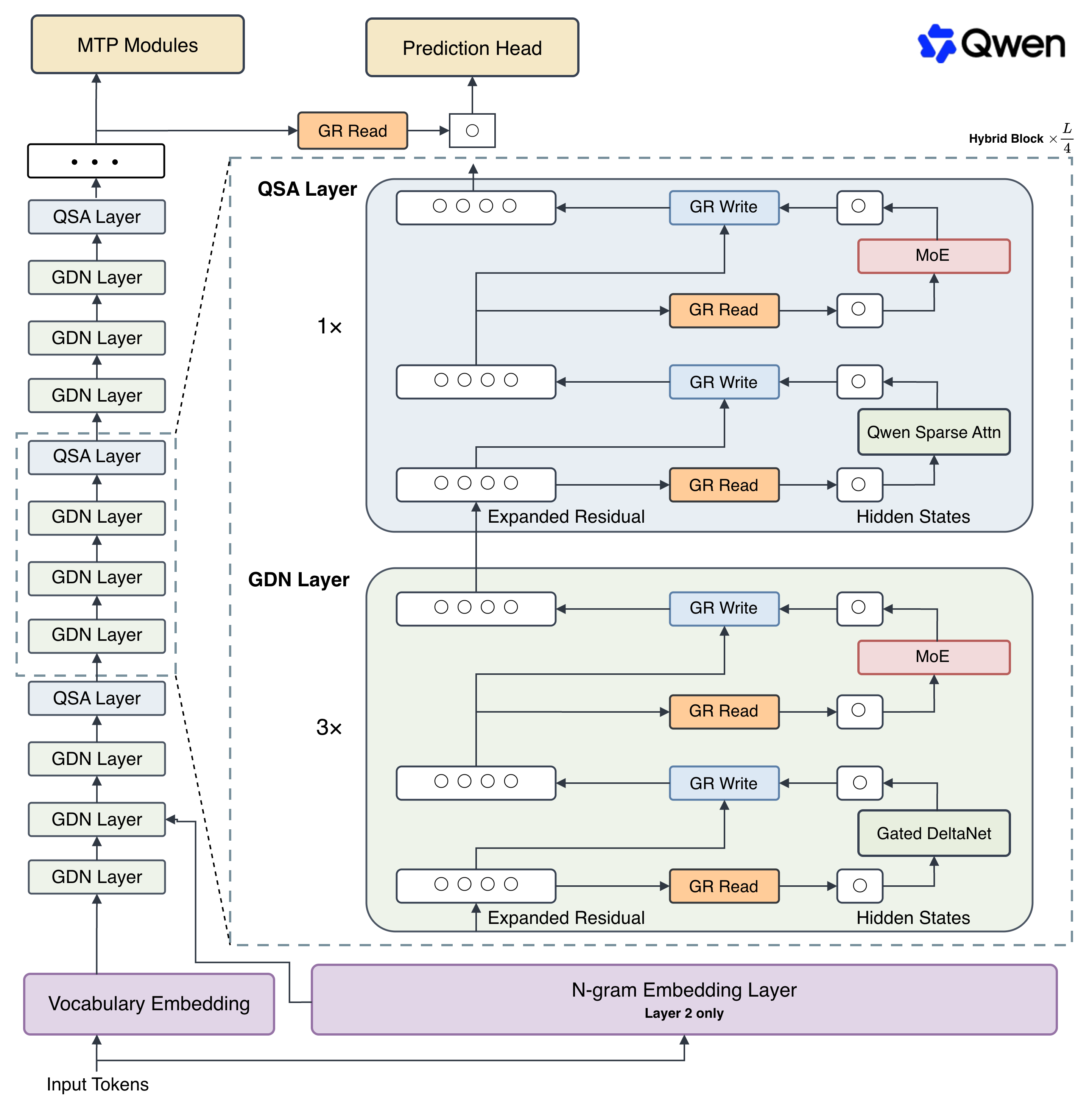
Core Idea: Inherits DSA's "Lightweight Indexer + Top-K Selection" paradigm, but elevates the selection unit from token to 4-token micro-block—first roughly screens Top-512 blocks at the block level, then losslessly expands back to tokens, extracting full-precision K/V from the original KV Cache, and performing standard sparse GQA precision calculation on a ~2K candidate set. Indexing overhead drops to 1/4 of DSA, with zero final attention precision loss.
Summary of QSA
QSA = Block-level coarse screening (Lightweight Indexer, Top-512 micro-blocks) → Lossless expansion (+ mandatory splicing of incomplete tail block) → Extract full-precision KV from original Cache → Standard GQA on constant-level candidate set. Compressed block keys are "signposts" throughout, never participating in final attention calculation.
1. Why QSA Exists
- DSA's pain point is Token-level indexing is too expensive:
- Lightning Indexer must score and rank each visible token individually, and when context grows to millions, the indexing unit's own linear scan cost becomes不可忽视.
- IndexCache-style cross-layer shared indexing schemes bet on "similar attention distribution between adjacent layers," but in GDN + Attention interleaved mixed architectures, the attention distributions of these two layer types differ greatly, making this assumption invalid.
- QSA's solutions (two points):
- Elevate selection unit to "4-token micro-block": Scoring objects change from tokens to blocks, directly dividing indexing overhead by 4.
- Independent compression and selection per layer: Independent of cross-layer attention similarity, naturally适配 GDN + Attention interleaved architectures.
2. QSA Position in Model (GDN + QSA Mixed Architecture)
GDN efficiently "remembers", QSA precisely "finds".
- Qwen3.8-Flash-Next has 48 layers, arranged in 3:1:
- 36 layers: Gated DeltaNet (linear attention, maintains fixed-size state matrix, no growth-type KV Cache generated)
- 12 layers: QSA (only layer generating growth-type KV Cache)
- Full attention layers in MTP (Multi-Token Prediction) module are also replaced by QSA.
- Context: Native 262,144 tokens, YaRN extrapolated to 1,000,000.
┌───────────────────────────────────────────┐
│  Layer 1  (GDN)   Fixed state S, no KV growth   │
│  Layer 2  (GDN)                                │
│  Layer 3  (GDN)                                │
│  Layer 4  (QSA)   ★ Growth-type KV Cache + Block-level filtering │
│  ...        Every 4 layers repeat ...               │
│  Layer 48 (QSA)                                │
└───────────────────────────────────────────┘
        36 layers GDN : 12 layers QSA = 3 : 1
3. QSA Core Architecture Design
QSA's essence: After the Lightweight Indexer selects Top- micro-blocks via "block-level coarse screening", it does NOT directly use compressed block keys for final attention calculation, but instead undergoes a precise "Restore → Assemble → Calculate" process.
Overview
Visible Prefix (Up to 1M tokens)
        │
        ▼
┌──────────────────────────────┐
│ ① Lightweight Indexer           │
│  - 4 tokens per micro-block     │
│  - Block-internal K mean → normalize│
│  - RoPE (using first token position)          │
│  - Multi-head ReLU scoring, Top-512 │
└──────────────────────────────┘
        │  512 block IDs (mere "signposts", not data)
        ▼
┌──────────────────────────────┐
│ ② Expand + Splice Tail          │
│  - 512 blocks → 2048 token indices │
│  - Unconditionally splice current incomplete block (0~3) │
└──────────────────────────────┘
        │  Sparse candidate set S_i (≤ 2051 tokens)
        ▼
┌──────────────────────────────┐
│ ③ Extract full-precision K/V from Original KV Cache │
│  (vLLM/SGLang extracts precisely by index) │
└──────────────────────────────┘
        │
        ▼
┌──────────────────────────────┐
│ ④ Standard Sparse GQA Precision Calculation          │
│  Softmax(Q·K_sparseᵀ/√d_k)   │
│  → Weighted aggregation V_sparse                   │
└──────────────────────────────┘
① Lightweight Indexer: Block-level Coarse Screening
Group the visible prefix into blocks of 4 tokens. Compress each complete micro-block into a "block key," then score against current Query:
complete_blocks = group(visible_prefix, block_size=4)    # One block per 4 tokens
block_keys      = mean(keys in each complete block)       # Block-internal K mean pooling
# → normalize → RoPE(first token position)
scores          = sum(relu(query_head @ block_key)        # Multi-index head scoring summation
                      for each indexer head)
selected_blocks = top_k(scores, k=512)                    # Select 512 blocks
attention_input = flatten(selected_blocks)                # Expand back to token positions
                  + current_incomplete_block              # + Incomplete tail block
- Scoring formula follows DSA Lightning Indexer's ReLU multi-head idea (no Softmax), but targets change from tokens to blocks.
- RoPE uses first token position within the block: Mean pooling blurs position info; using first token position injects a coarse-grained positional signal into the block key of "roughly where this entire block lies on the time axis."
- Budget conversion: 2048 token budget ÷ 4 token/block = max 512 complete blocks.
- Block keys only for scoring: Compression here is "lossy," but it serves only as a signpost, not entering final attention.
Original K sequence (visible prefix, millions of tokens):
[k₁ k₂ k₃ k₄ | k₅ k₆ k₇ k₈ | ... | kₘ kₘ₊₁]
  └─ Block 1 ─┘    └─ Block 2 ─┘           └ Tail block (incomplete)
      ↓ Mean Pooling         ↓
  [ k̃₁ ]         [ k̃₂ ]   ...     (Tail block not pooled, unconditionally retained)
      ↓ RoPE(first token position)
      ↓
  Score against Query → Top-512 blocks
② Index Expansion and Tail Assembly (Expand & Assembly)
- Token-level restoration: 512 block IDs losslessly unpack back into 2048 high-precision token position indices.
- Tail mandatory splicing (Tail Integration): The last micro-block is often incomplete (containing 0~3 tokens). These are nearest to current Query information (local syntax, coherence dependencies). They cannot be missed because their block didn't rank in Top-512 → unconditionally spliced in, ensuring causal mask completeness.
- Final candidate set: tokens, far smaller than the full million-token context.
512 block IDs ──Expand──→ 2048 token indices
                              │
                              +  Incomplete tail block (0~3, unconditionally spliced)
                              │
                              ▼
                        S_i ≤ 2051 positions
Compared to DSA: DSA ranks tokens independently, no need for block tail rules—this is one of the direct differences between "selecting blocks" vs "selecting tokens."
③ Extract Full-Precision Data from Original KV Cache
- Key Point: Compressed block keys act only as "signposts", never participating in final attention from start to finish.
- VRAM always stores complete, uncompressed K/V Cache (QSA compresses computation and indexing, not storage content—distinct from CSA/HCA).
- After determining ~2K positions, the inference engine (vLLM/SGLang) precisely extracts corresponding token full and from HBM by index.
- KV read volume per query is constrained to constant ~2K, synchronizing memory access bottleneck relief.
④ Execute Standard Sparse Attention Calculation (Sparse GQA)
Upon obtaining ~2K full-precision K/V, run completely standard GQA matrix operations on the candidate set (QSA layer internally adopts GQA head structure):
1. Attention Scores (Softmax):
Softmax normalizes only on ~2051 positions—attention weights recapitulate competition within the selected set; weights for discarded tokens are strictly 0.
2. Weighted Value Aggregation:
Since and are original full-precision vectors, no approximation error exists on selected tokens; precision loss can only come from "selecting wrong blocks" (cost of block-level coarse screening, see §5).
4. Complexity Analysis (1M Context, Single Query Perspective)
| Step | Standard Attention | DSA (token-level) | QSA (block-level) |
|---|---|---|---|
| Index Scoring | — | ||
| Attention Computation | |||
| KV Read Volume | All | 2048 tokens | 2048~2051 tokens |
| KV Storage | (does not compress storage) | (does not compress storage) |
- Core Attention cost: QSA equals DSA (both constant-level).
- Indexing cost: QSA is 1/4 of DSA, relative advantage grows as increases.
- Mixed architecture bonus: KV Cache only 12/48 layers grow (GDN layers maintain fixed state), storage layer count naturally saves 4x.
Measured Effect (Qwen Official):
| Metric | Value |
|---|---|
| 1M Context Attention Kernel Acceleration | Prefill 7.6× / Decode 4.9× |
| 90% Prefix Cache Hit Scenario | Prefill throughput reaches 8.6× of Qwen3.7-Plus (1M context) |
5. QSA vs DSA vs NSA
| Scheme | Source | Selection Unit | Granularity | 2048 Budget Meaning | Tail Incomplete Block | Final Attention Data Used |
|---|---|---|---|---|---|---|
| NSA | DeepSeek | Large Blocks (512 tokens/block) | Coarse | Top-k blocks | Covered by sliding window branch | Original KV of selected blocks |
| DSA | DeepSeek V3.2 | Single Token | Fine | Max 2048 tokens | No corresponding rule | Original KV of selected tokens |
| QSA | Qwen3.8-Flash-Next | 4-token Micro-Block | Medium | Max 512 blocks | Unconditionally Directly Included | Original KV of selected blocks (+ tail) |
Evolutionary Logic: NSA Large Blocks "granularity too coarse, potentially harming a large area" → DSA Token-level "precise but expensive indexing" → QSA takes the middle point: 4-token micro-block, balancing indexing cost and selection precision.
QSA Block-level Selection Cost ("Harm"):
- Selecting 1 critical token will be linked with the other 3 tokens in its block (redundant, but softmax within candidate set will automatically lower its weight).
- Missing 1 block means missing all 4 tokens in it (theoretical precision loss at granularity level).
- Qwen's judgment: 4 is small enough that harm is limited; ÷4 saving in indexing overhead outweighs it.
Slide Window Attention (SWA)

SWA: Restrict each token's attention range
- Single-layer sliding window only sees local context
- But multi-layer stacking, with principles similar to CNN, information can propagate inter-layer to achieve dependencies beyond window range.
| Attention Type | Computational Complexity | Description |
|---|---|---|
| Causal Attention | Each token must compute attention scores with all historical tokens (L tokens × L historical positions × d_k dimension) | |
| Slide Window Attention | Each token only computes attention with tokens within the window (w = window size, typically 2048~32768) |
| Attention Type | KV Cache Memory | Description |
|---|---|---|
| Causal Attention | Need to cache Key/Value for all historical tokens (h = head count) | |
| Slide Window Attention | Theoretically only need to cache KV for recent tokens |
DefectAttention Sink
When using pure sliding window for ultra-long sequence inference, model performance drops drastically. Reasons:
- Initial tokens (e.g., prompt beginning) gradually slide out of window → permanently lost
- These tokens often contain critical context (e.g., instructions, role settings)
- Model loses "anchor", leading to generation quality collapse
Fix Solutions
1. StreamingLLM
Retain KV Cache for first tokens (sink tokens), while using sliding window for subsequent tokens:
2. Hybrid Attention
- Method 1: Combine sliding window (local) and global attention in a 1:1 ratio
- Method 2: Interpolate only 1 global attention layer for every 5 local attention (sliding window) layers
Infini-attention
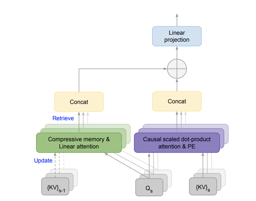
Principle
1. Compressing Long-term Memory (Recursive Update)
For the -th token, update compressed memory and normalized vector as follows:
- : Forgetting Factor (learnable scalar), controls history memory decay rate
- : Strong forgetting, only retain recent context
- : Weak forgetting, long-term memory accumulation (but numerical overflow prevention needed)
- : Feature Mapping Kernel Function, maps Key to linear attention space
- Standard choice: (ensures non-negativity, stabilizes training)
- dimension fixed at (independent of sequence length ) → Bounded Memory Guarantee
2. Long-term Attention Calculation
- Numerator : Interaction between compressed memory and current Query
- Denominator : Normalization term (avoids numerical instability)
- Computational Complexity: (independent of ) → Supports infinite-length sequences
3. Local Attention & Long-term Attention Fusion - Gating Mechanism
Local attention and long-term attention fuse via sigmoid gating:
- : Learnable scalar parameter (initialized to 0)
- : Rely fully on local attention (short context scenarios)
- : Rely fully on compressed memory (ultra-long context scenarios)
- Adaptive Training: Model automatically learns optimal fusion ratio under different tasks/lengths
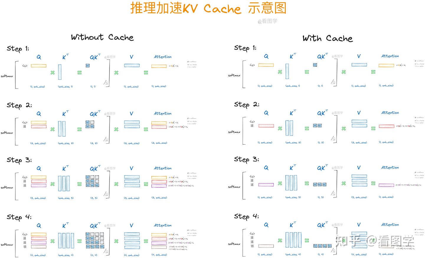
KV Cache
MTP (Multi-Token Prediction)
1. Blockwise Parallel Decoding (Google, NeurIPS 2018)
📄 Blockwise Parallel Decoding for Deep Autoregressive Models Focus: Inference Acceleration
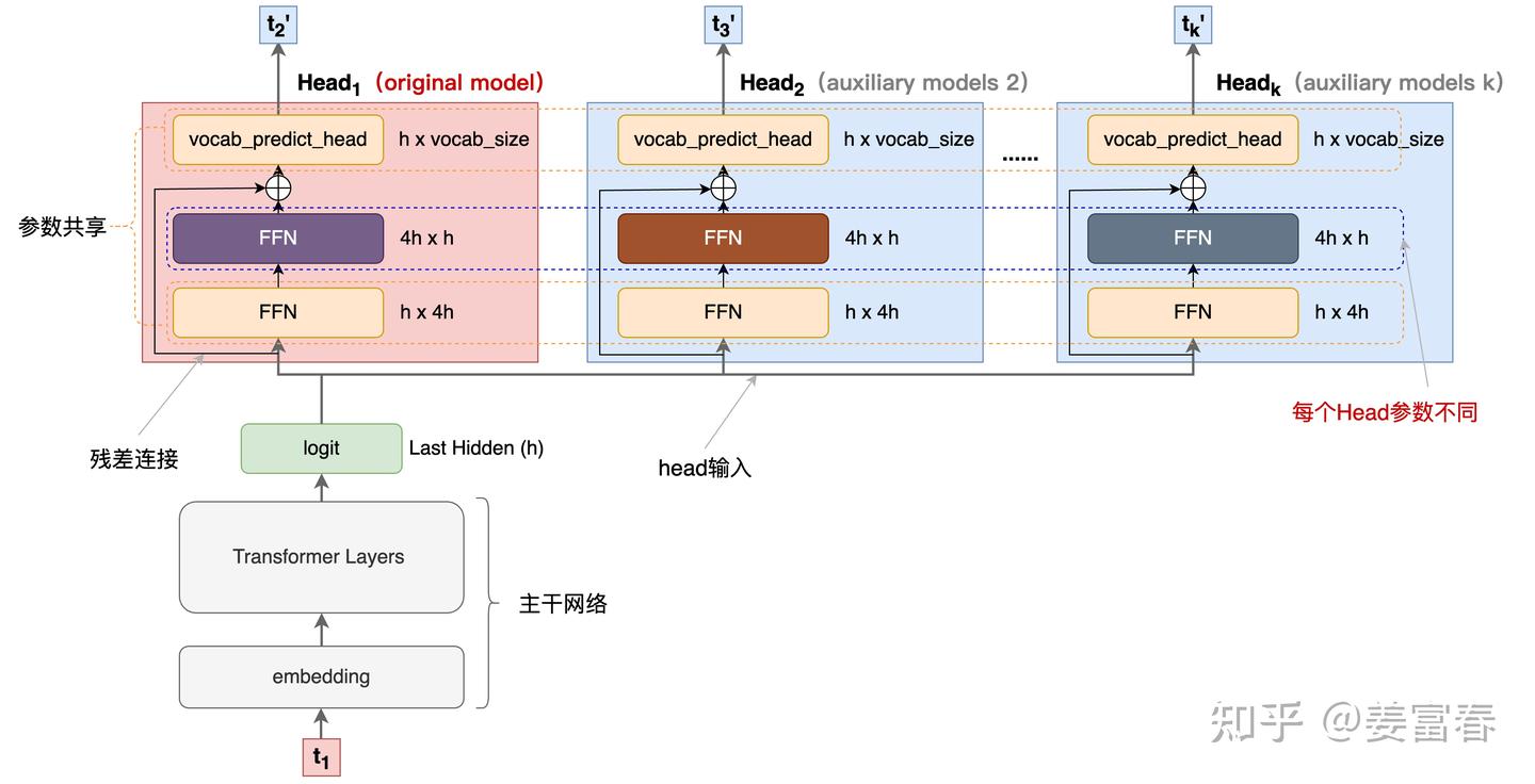
Network Structure:
Key Structural Points:
| Component | Shared? |
|---|---|
| First FFN Layer (h→4h) | ✅ Shared |
| Second FFN Layer (4h→h) | ❌ Independent per Head |
| Vocabulary Projection + Softmax | ✅ Shared (original model's) |
Inference Three Stages:
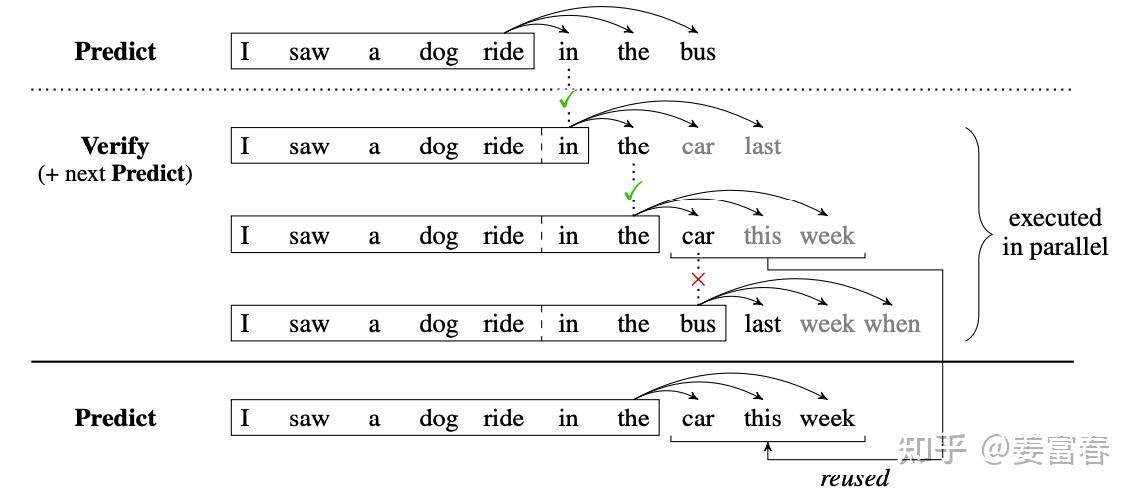
- Predict: k Heads generate k tokens simultaneously
- Verify: Concatenate sequence + generated tokens as k
<sequence_input, label>pairs, batched into Head₁ for verification - Accept: Accept the longest k tokens where Head₁ prediction matches label
Acceleration Analysis (assuming all auxiliary heads predict correctly):
| Scheme | Inference Steps | When k=4 |
|---|---|---|
| Token-by-token | m | 1× |
| Non-overlapping 3-stage | 2m/k | 2× |
| Predict & Verify Overlap | 1+m/k | ≈3.2× |
⚡ GPU parallelism makes: single sequence vs batch sequence, single head vs multi-head computation time differences negligible; bottlenecks lie in memory access, not computation.
2. Meta's MTP (Meta, April 2024)
📄 Better & Faster Large Language Models via Multi-token Prediction Focus: Training + Inference Dual Optimization
Network Structure:
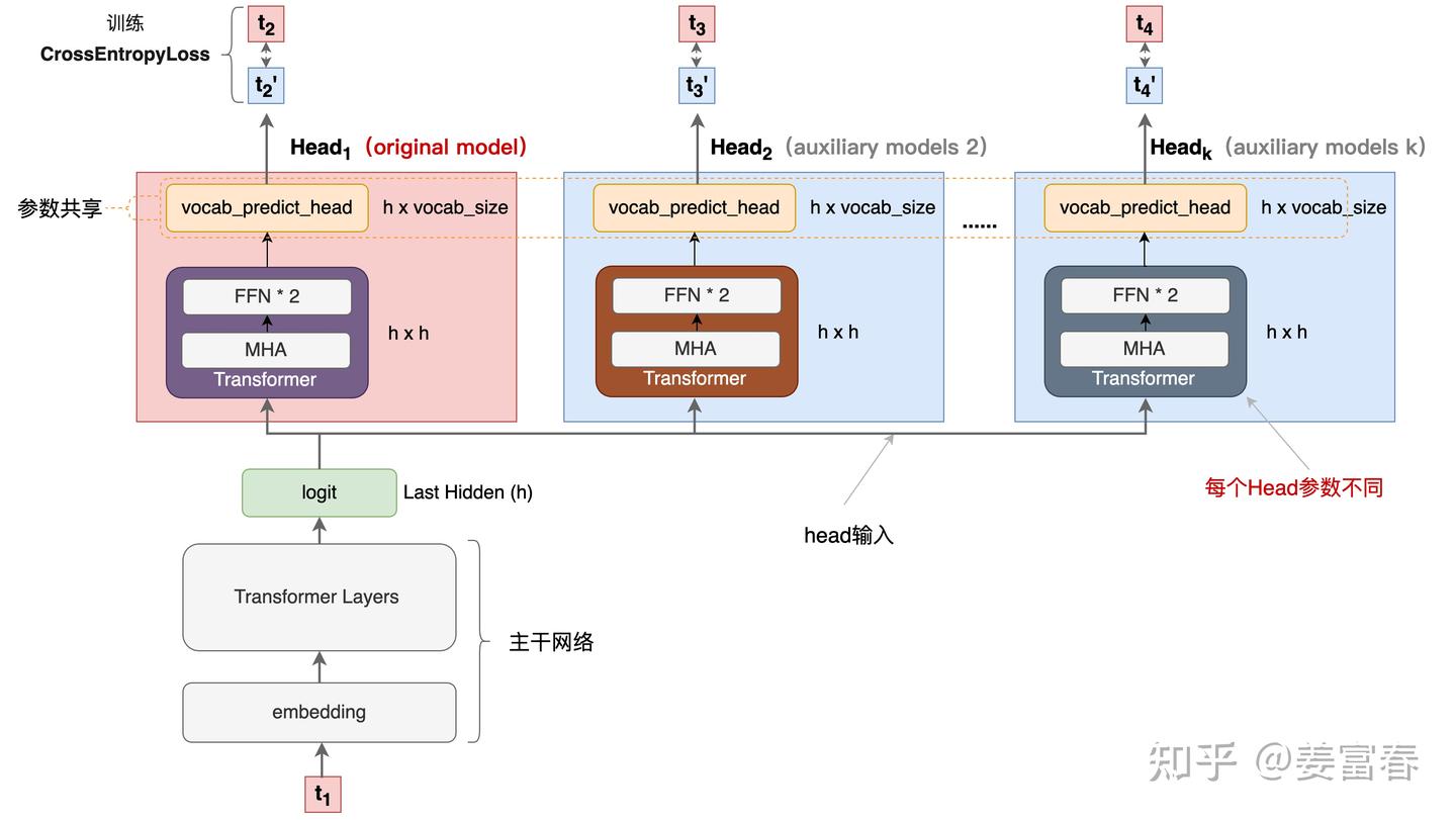
Differences from Blockwise Parallel Decoding (very minor):
- Head Internal Structure: 2 FFN layers → Complete Transformer Layer (MHA+FFN)
- New focus on training acceleration (multiple heads compute loss in parallel, improving sample efficiency)
⚠️ Key Commonality: Heads are independent, no information transmission.
3. DeepSeek MTP (DeepSeek, Dec 2024)
📄 DeepSeek-V3 Focus: Training acceleration primarily, inference secondary
Most fundamental difference from previous methods: Causal Chain Connection—each prediction Module links sequentially, information progressively transmitted.
3.1 MTP Module Implementation
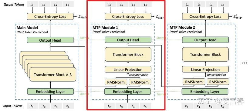
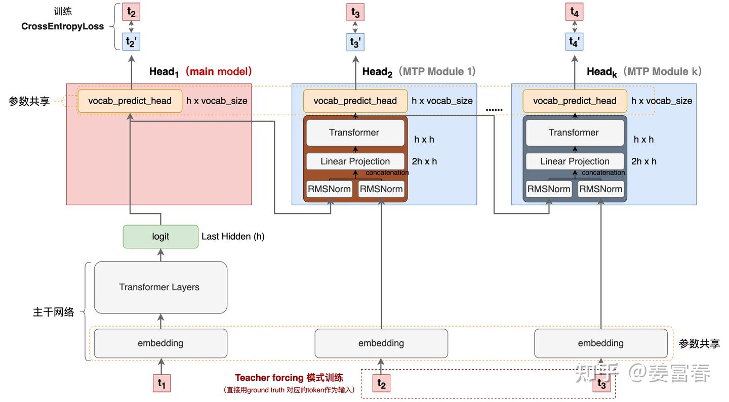
3.2 Training Sample Construction
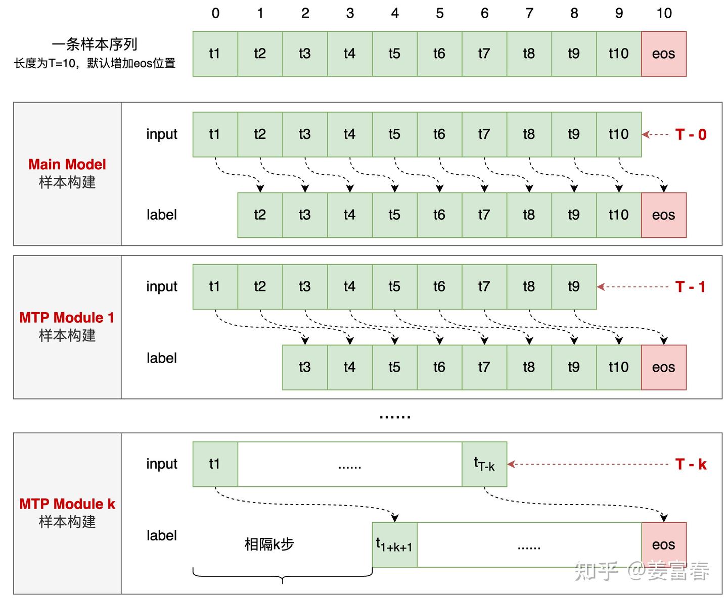
3.3 Inference Method
Method 1: Delete MTP heads → degenerates to ordinary LLM inference, no acceleration.
Method 2: Self-Speculative Decoding (similar to Blockwise 3-stage)
- Predict: k Modules generate k tokens simultaneously (Free-Running mode)
- Verify: Concatenate sequence, batch into Main Model for verification
- Accept: Accept longest token sequence verified successfully
Note: During inference, Emb() uses embeddings of predicted tokens, not ground truth. </translate_input>